The Models We Choose Define the Worlds We Can See
Modeling is commonly framed as approximation — the assumption that a system exists in full, and our models trace its contours with varying levels of fidelity.
This framing is incomplete.
Models do not merely approximate reality with varying precision. They constrain what dynamics can be represented in the first place. A model that represents populations as aggregate compartments cannot express phenomena that depend on individual interactions. A model that represents individuals on networks cannot yield closed-form predictions. These are not differences in accuracy — they are differences in what the model is capable of saying.
Models define the space of representable dynamics, and therefore constrain what can be observed, predicted, and decided.
This essay develops this claim through epidemic modeling. We begin with compartmental models (SIRS), introduce agent-based models as a different representational class, establish their formal relationship, and then show — through four computational experiments — that the choice of model determines not only what dynamics emerge, but which interventions can be evaluated.
From Curves to Computations
Consider a familiar tool: compartmental epidemic models. The SIRS model divides a population into Susceptible, Infected, and Recovered groups, with transitions governed by differential equations [1].
The SIRS model does not represent individuals, interactions, or behavior explicitly. Instead, it encodes:
- Infection as a rate ($\beta$)
- Recovery as a rate ($\gamma$)
- Loss of immunity as a rate ($\omega$)
The system is governed by:
$$ \frac{dS}{dt} = -\frac{\beta S I}{N} + \omega R $$$$ \frac{dI}{dt} = \frac{\beta S I}{N} - \gamma I $$$$ \frac{dR}{dt} = \gamma I - \omega R $$where $N = S + I + R$ is conserved.
This reflects a mean-field assumption: individuals mix homogeneously, and interactions can be averaged into continuous flows [2].
This imposes specific constraints on the model’s behavior.
Because the system evolves through ordinary differential equations in the variables $S(t)$, $I(t)$, and $R(t)$, its trajectories are continuous functions of time. Infection is represented as a continuous flow between compartments rather than as discrete transmission events between individuals.
The evolution of the system is fully determined by the current values of $(S, I, R)$ and the parameters $\beta, \gamma, \omega$. Given these values, the model produces a single trajectory (up to numerical error), rather than a distribution of possible outcomes arising from different interaction histories.
The model assumes that aggregate rates are sufficient statistics of the underlying process [2].
A Different Ontology
Now consider an alternative: an agent-based model (ABM).
Instead of compartments, we simulate individuals:
- Each agent has state (S, I, R)
- Each agent has attributes (behavior, movement, occupation)
- Each agent interacts locally with others
Instead of rates, we define rules.
Instead of equations, we define mechanisms.
# Pseudocode: Agent-Based Infection Step

for agent in population:
    if agent.state == INFECTED:
        for neighbor in agent.get_contacts():
            if neighbor.state == SUSCEPTIBLE:
                if random() < transmission_probability(agent, neighbor):
                    neighbor.state = INFECTED

    if agent.state == INFECTED:
        if random() < recovery_probability(agent):
            agent.state = RECOVERED
Agent-based models are widely used to study infectious disease dynamics precisely because they allow heterogeneous agents and structured interactions [3].
It is a different model class. The system is no longer defined by aggregate compartments, but by individual agents, their attributes, and the interaction rules that govern their behavior. The state of the system therefore includes not only how many individuals are infected, but also who is infected, how they are connected, and how they interact.
Agent-Based Models as Computational Systems
To understand why relaxing mean-field assumptions has such consequences, it is useful to situate agent-based models within a broader computational framework.
Cellular automata (CA) are among the simplest systems that exhibit this property. A cellular automaton consists of discrete cells arranged on a grid, each holding a finite state value. At each time step, every cell updates its state according to a fixed local rule that depends only on its current state and the states of its immediate neighbors [8].
Despite their simplicity, cellular automata produce global patterns that depend on the repeated application of local update rules. Wolfram’s classification of elementary cellular automata demonstrated that even one-dimensional systems with binary states and nearest-neighbor rules can produce behavior ranging from fixed points to structures that are computationally irreducible — meaning the only way to determine the system’s state at time $t$ is to execute all $t$ steps of the computation [7].
Agent-based models generalize this framework in three directions:
- From regular grids to arbitrary graphs. Agents interact through network topologies — small-world, scale-free, multilayer — rather than fixed lattice neighborhoods.
- From uniform rules to heterogeneous agents. Each agent can carry distinct attributes (age, occupation, behavior) that modulate its update rule.
- From fixed rules to adaptive behavior. Agents can change their rules in response to local or global state — complying with interventions, altering contact patterns, or developing immunity.
These extensions preserve the core computational property: the system evolves through the iterated application of local rules, and global behavior emerges from the sequence of interactions rather than from a closed-form expression over aggregate variables [3][8].
This has a direct consequence for predictability. When the mean-field assumptions hold — homogeneous mixing, statistical independence, no persistent structure — the system’s expected trajectory can be computed analytically. The aggregate ODE is a sufficient summary. But when these assumptions are relaxed, the system inherits the computational properties of its underlying interaction structure. Behavior becomes sequence-dependent: the order in which agents interact, the specific paths through which infection propagates, and the local clustering of states all influence the outcome in ways that cannot be shortcut.
Once a system is represented as local rules executed over time, its behavior depends on the sequence of state transitions those rules generate, rather than on a closed-form expression over aggregate variables.
The experiments that follow test this boundary systematically — first confirming that agent-based models recover ODE dynamics under restricted assumptions, then showing where and why the equivalence breaks down.
Recovering the Familiar
To make this concrete, we begin with an experiment.
We construct an agent-based model that mirrors the assumptions of SIRS:
- Homogeneous agents
- Random mixing
- Fixed transition probabilities
# Pseudocode: Homogeneous ABM approximating SIRS

for timestep in simulation:
    shuffle(population)

    for agent in population:
        contacts = random_sample(population, k=CONTACT_RATE)

        for other in contacts:
            attempt_infection(agent, other)

        attempt_recovery(agent)
        attempt_resusceptibility(agent)

    record_global_counts(S, I, R)
When we aggregate the results, the system reproduces the characteristic dynamics of compartmental models.
This aligns with established results:
Under homogeneous mixing and large populations, agent-based simulations converge to mean-field models such as SIR/SIRS [4].
The following figure shows the result: an ensemble of 20 ABM runs (colored bands showing ±1 standard deviation) overlaid on the deterministic SIRS ODE solution (white dashed curves). The ABM mean closely traces the ODE prediction throughout the simulation, confirming that under homogeneous mixing, the agent-based model recovers compartmental dynamics. The peak infection reaches approximately 31% of the population around day 25.
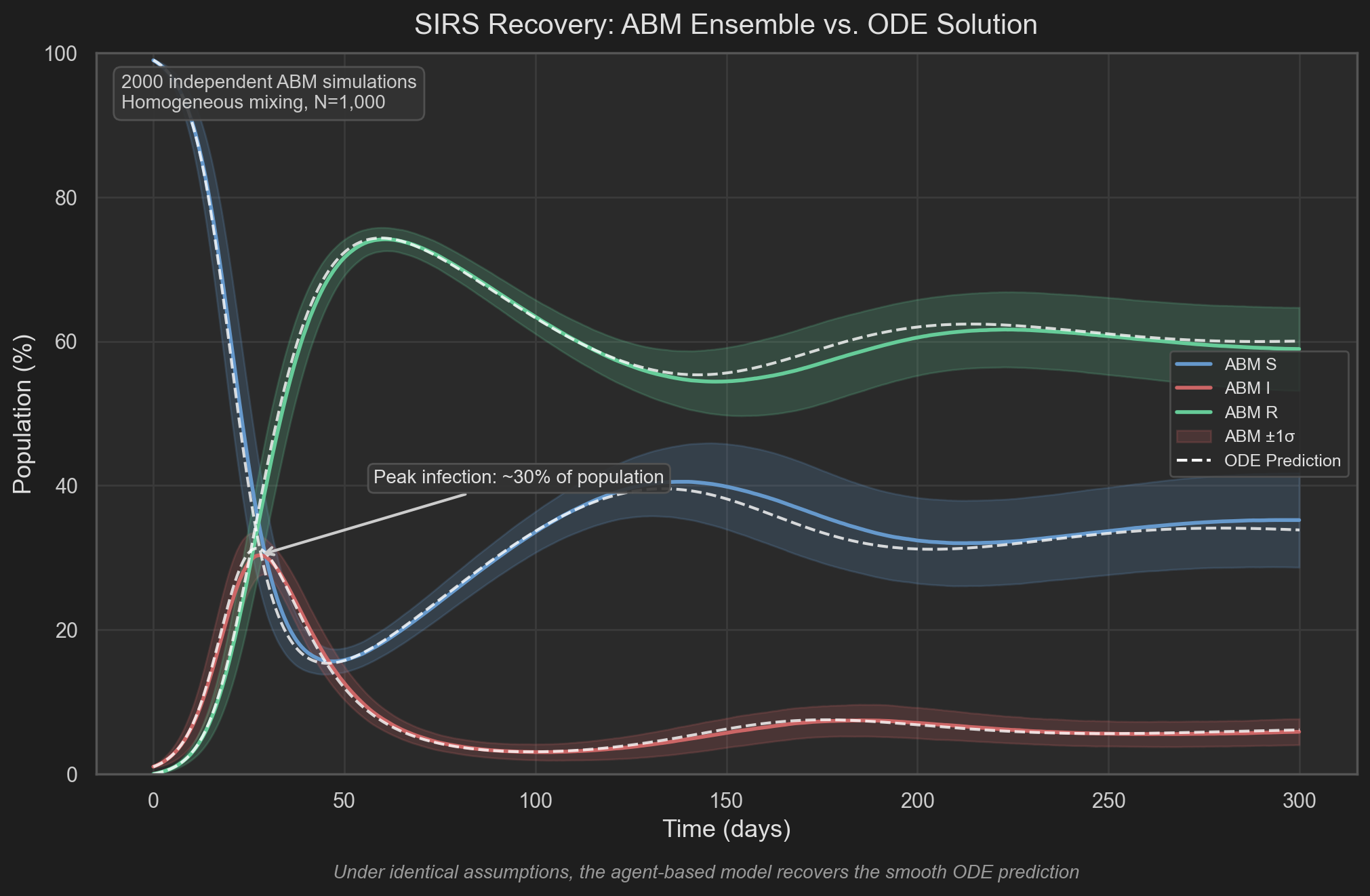
This is our first key result: compartmental models can be understood as coarse-grained limits of underlying individual-based processes.
From Agent-Based Dynamics to Mean-Field Equations
The recovery experiment demonstrated empirically that an agent-based model reproduces SIRS dynamics under homogeneous mixing. We can make this relationship precise by deriving the SIRS equations as a limiting case of agent-level dynamics.
Consider a population of $N$ agents, each in state $S$, $I$, or $R$. At each time step, every agent contacts $k$ other agents drawn uniformly at random. For a susceptible agent making a single contact, the probability that the contact is infected is:
$$ P(\text{contact is infected}) = \frac{I}{N} $$If each contact transmits infection independently with probability $\beta'$, the probability that a susceptible agent with $k$ contacts avoids infection entirely is:
$$ P(\text{not infected}) = \left(1 - \frac{\beta' I}{N}\right)^k $$For small $\beta' I / N$, this can be approximated:
$$ P(\text{infected}) \approx \frac{\beta' k I}{N} $$The expected number of new infections per time step among all susceptible agents is therefore:
$$ \mathbb{E}[\Delta I_{\text{new}}] \approx \frac{\beta' k \cdot S \cdot I}{N} $$Defining $\beta = \beta' k$ and taking the continuous-time limit, we recover the SIRS infection term:
$$ \frac{dI}{dt} \bigg|_{\text{infection}} = \frac{\beta S I}{N} $$The recovery and immunity loss terms follow analogously from individual transition probabilities $\gamma$ and $\omega$.
This derivation rests on four explicit assumptions:
- Homogeneous mixing. Every agent is equally likely to contact every other agent. There is no network structure, no spatial locality, and no persistent contact relationships.
- Statistical independence. Each contact event is independent. The probability of infection does not depend on the agent’s contact history or the states of other contacts.
- No structural heterogeneity. All agents have the same contact rate $k$ and the same transmission probability $\beta'$. There are no high-degree hubs, no behavioral variation, and no demographic stratification.
- Expectation replaces distribution. The derivation uses expected values rather than the full distribution of outcomes. Stochastic variation across runs — which depends on the specific sequence of interactions — is averaged away.
Under these assumptions, the SIRS equations are the expected-value projection of the agent-based dynamics. The ODE variables $(S, I, R)$ are sufficient statistics for the system state, and the aggregate trajectory is determined by the parameters $(\beta, \gamma, \omega)$ alone.
SIRS is the expected-value projection of a restricted class of agent-based systems. Each assumption removed opens a degree of freedom that the ODE cannot represent.
The remaining sections test what happens when these assumptions are relaxed.
Where Do the Parameters Live?
The difference comes down to where parameters live in each model.
In SIRS, parameters are global:
- $\beta$ summarizes infection dynamics
- $\gamma$ summarizes recovery
- $\omega$ summarizes immunity loss
These are not mechanisms—they are effective parameters, aggregating many micro-level processes [2].
In agent-based models, parameters are local:
- Contact networks
- Behavioral rules
- Movement constraints
- Context-dependent interactions
Here, parameters do not summarize computation.
They define the computation itself.
Macro-level parameters often emerge from micro-level rules rather than exist independently [5].
Breaking the Equivalence
We relax the three assumptions from the derivation section and observe what changes.
We introduce:
- Network structure (e.g., small-world or scale-free graphs)
- Behavioral heterogeneity
- Occupation-dependent exposure
# Pseudocode: Structured Interaction

for agent in population:
    contacts = agent.network_neighbors()

    for neighbor in contacts:
        if interaction_occurs(agent, neighbor):
            attempt_infection(agent, neighbor)
When we simulate this system, the model produces behaviors that cannot be represented by the original SIRS formulation:
- Infections can remain confined within densely connected subgraphs rather than spreading uniformly
- Transmission rates vary across individuals depending on their position in the network
- Repeated simulations with identical aggregate initial conditions produce different trajectories due to stochastic interaction patterns
Network structure can fundamentally alter epidemic dynamics, producing outcomes not captured by homogeneous mixing models [6].
The left panel shows the recovery experiment for reference—agents mixing randomly produce dynamics that match the ODE. The right panel tells a different story: when agents are placed on a scale-free network with heterogeneous transmission rates, individual simulation trajectories (thin colored lines) spread widely around the ODE prediction (white dashed). Some runs produce large outbreaks, others fizzle early. The smooth ODE curve cannot capture this trajectory diversity.
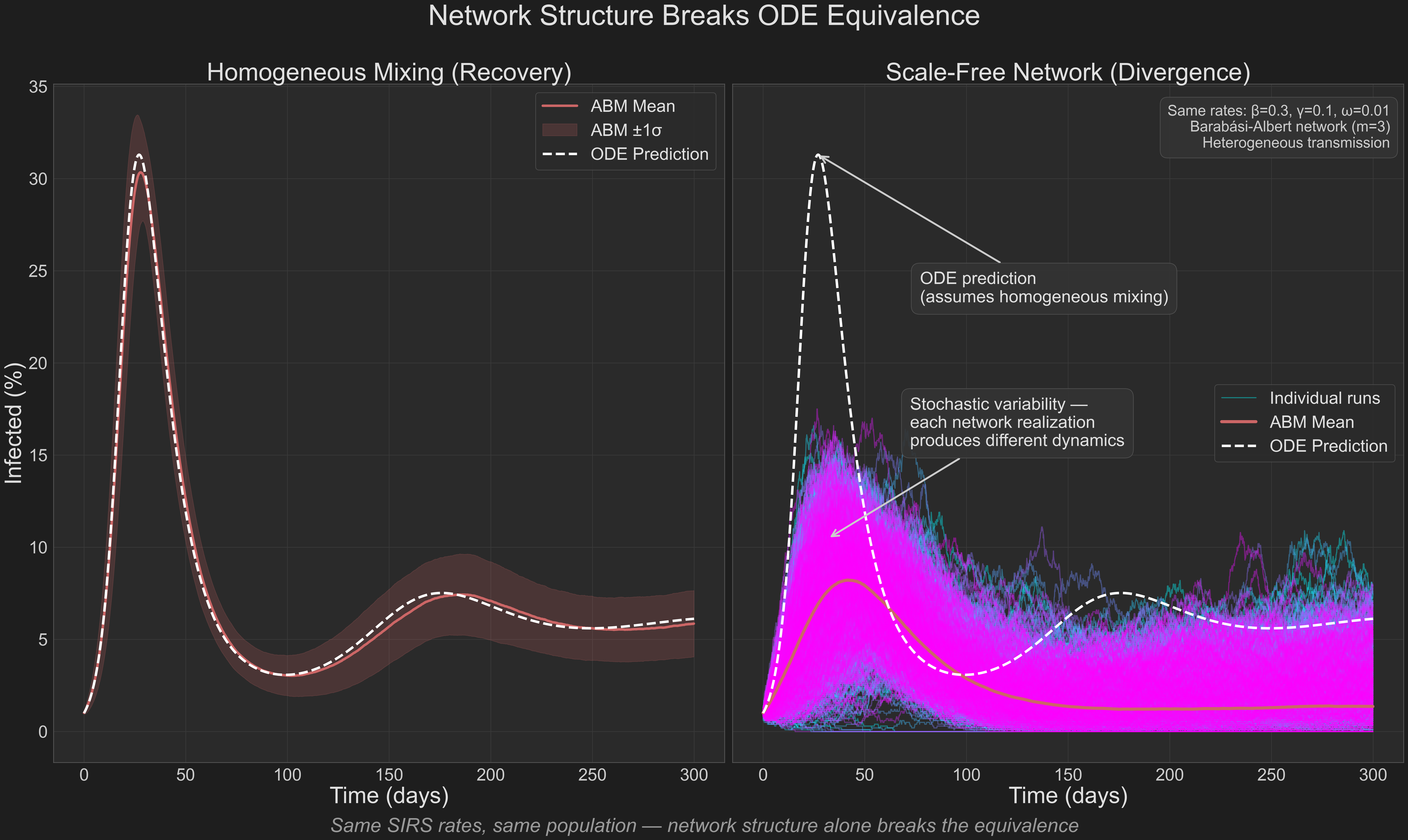
At this point, the SIRS framework cannot be “retuned” to match the behavior.
The SIRS formulation lacks variables for network position or interaction history — retuning parameters cannot recover what the model doesn’t encode.
Irreducibility and the Limits of Compression
A system is computationally reducible if there exists a shortcut — a closed-form expression that maps parameters and initial conditions to outputs without executing each step of the dynamics. The SIRS model is reducible in this sense. Given $(\beta, \gamma, \omega, N, I_0)$, the full trajectory is determined by integrating three ODEs.
Certain systems cannot be predicted without simulating their step-by-step evolution [7].
The agent-based model under network structure is not reducible in this way. Non-compliance modulates per-contact transmission probability at the agent level. The infection cascade that follows depends on which specific agents interact in which order — which high-degree nodes are contacted early, which clusters saturate before the infection front arrives, which transmission paths activate before local immunity accumulates. No closed-form expression over $(\beta, \gamma, \omega, N, \rho)$ can recover it.
We can probe this directly by sweeping non-compliance rate $\rho \in [0, 1]$ and recording peak infection across 200 simulation runs per level:
# Pseudocode: Sensitivity Experiment

for non_compliance_rate in [0.2, 0.4, 0.6, 0.8]:
    configure_population(non_compliance=non_compliance_rate)
    run_simulation()
    record_outcomes()
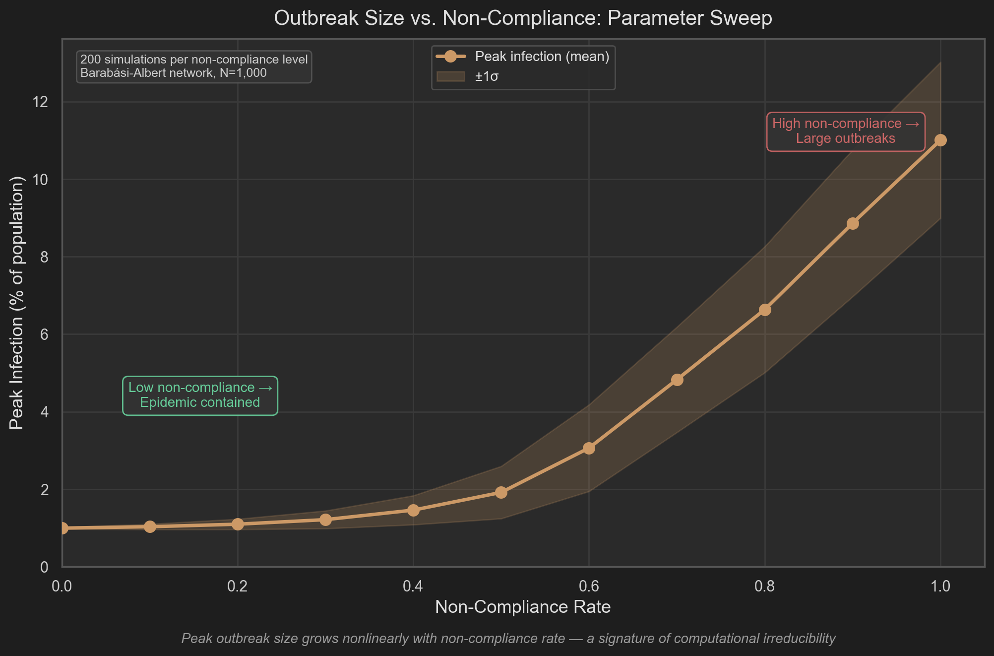
The mean curve shows peak outbreak size growing nonlinearly with $\rho$. But the mean is not the primary signal — the band is.
At each non-compliance level, 200 runs with identical aggregate parameters produce a distribution of outcomes. This variance is not numerical noise. It is information carried by the specific sequence of agent interactions in each run: which agents contacted which, in what order, through which network paths. The aggregate parameters $(\beta, \gamma, \omega, \rho)$ do not determine it.
A computationally reducible system has no such residual. Given the parameters, the output is fixed — as it is in SIRS. The band in the figure is a direct measurement of that residual: the portion of the outcome that lives in the interaction sequence and cannot be compressed into any aggregate summary.
When Structure Determines the Answer
The previous experiments follow a single thread: each step removes a representational degree of freedom.
- An agent-based model reproduces SIRS dynamics under homogeneous mixing
- Introducing interaction structure produces divergent trajectories
- System behavior depends on the sequence of interactions, not just aggregate state
The remaining question is whether these losses affect decisions.
This can be tested by comparing intervention strategies that depend on interaction structure.
Experimental setup
We consider two vaccination strategies:
- Random vaccination: immunize 20% of the population uniformly at random
- Targeted vaccination: immunize the 20% most-connected individuals (highest-degree nodes)
Both strategies are evaluated under:
- identical disease parameters ($\beta = 0.3, \gamma = 0.1, \omega = 0.01$)
- identical population size ($N = 1000$)
- identical initial conditions
The only difference between models is how interactions are represented:
- Homogeneous model: agents mix uniformly; degree is not defined
- Structured model: agents interact through a layered contact network with heterogeneous degree distribution
Representational constraint
In the homogeneous model, all agents have identical expected contact rates.
Formally, for any two agents $i, j$:
$$ \mathbb{E}[\text{contacts}_i] = \mathbb{E}[\text{contacts}_j] $$There is no variable in the model that distinguishes highly connected individuals from others.
As a result:
- “highest-degree node” is undefined
- targeted vaccination reduces to random vaccination
The two interventions are therefore identical within the model.
Structured model behavior
In the structured model, each agent has a defined contact set:
$$ k_i = |\text{neighbors}(i)| $$The distribution of $k_i$ is heterogeneous.
This introduces:
- high-degree nodes (hubs)
- clustered subgraphs (households, workplaces)
- repeated interactions within local neighborhoods
Targeted vaccination removes nodes with large $k_i$, reducing the number of potential transmission paths more than random removal.
Results
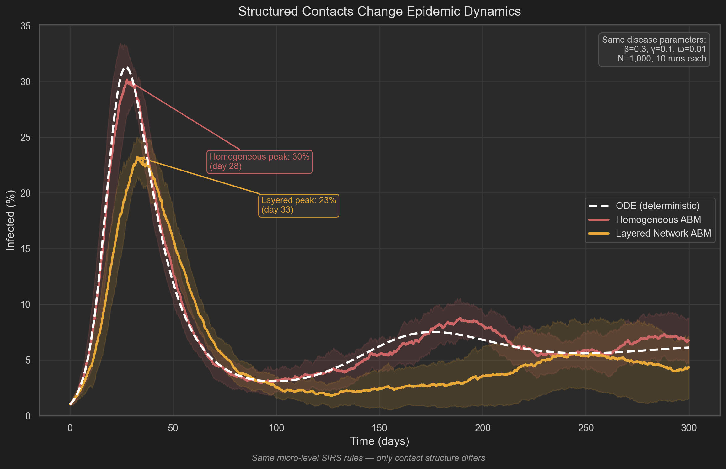
The trajectory comparison shows that introducing contact structure alone — without changing disease parameters — alters:
- peak timing
- peak magnitude
- equilibrium behavior
The structured model produces a lower and broader infection curve. This follows from local saturation effects: infections propagate within clusters before reaching the broader network.
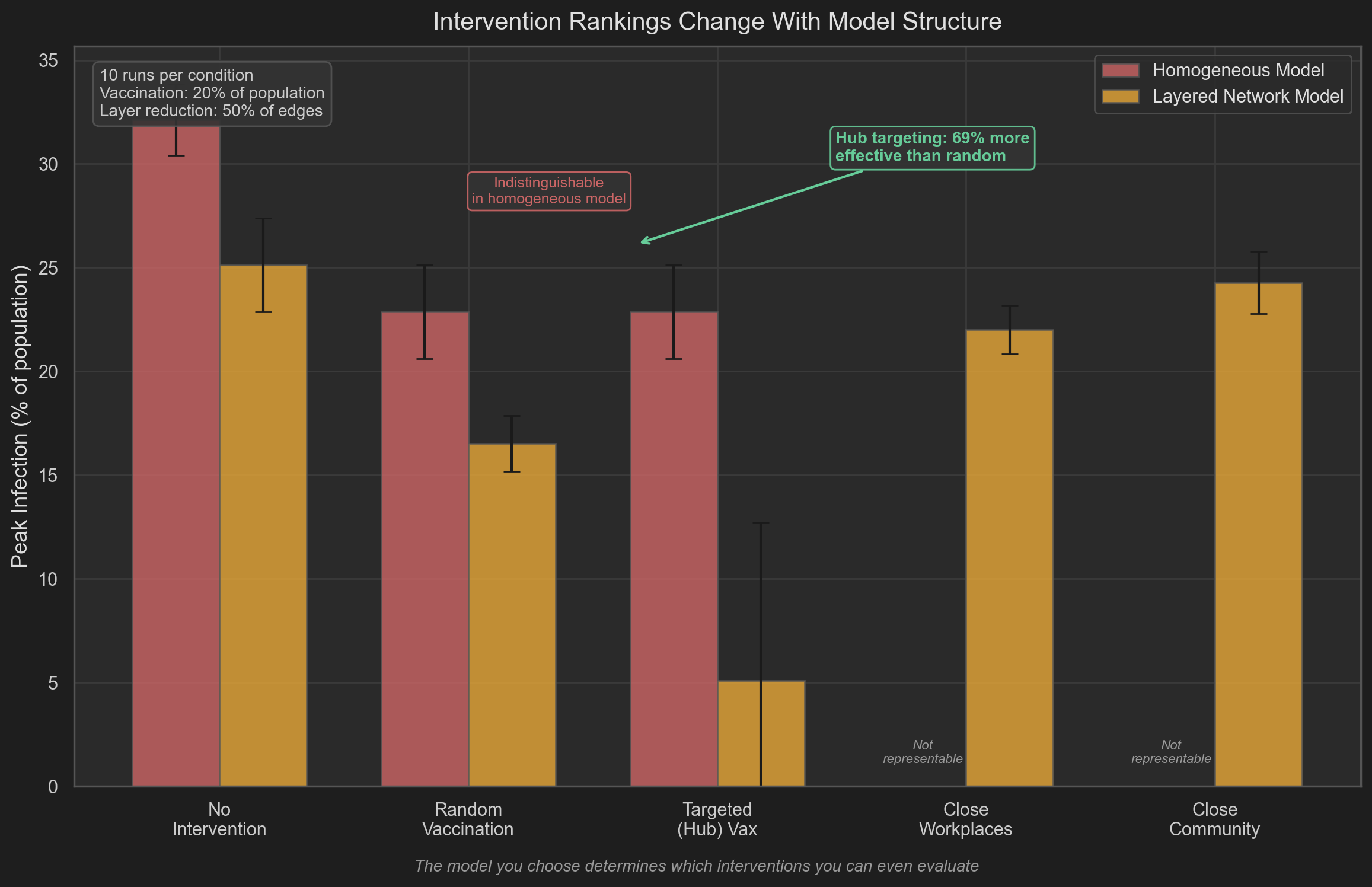
The intervention comparison shows a qualitative difference:
Homogeneous model:
- random vaccination ≈ targeted vaccination
- both reduce peak infection to approximately 23%
Structured model:
- random vaccination → moderate reduction
- targeted vaccination → peak infection reduced to ~5%
The difference arises from network structure, not from changes in disease parameters.
Interpretation
The homogeneous model produces a correct result within its assumptions: all agents are statistically identical, so intervention strategies that depend on heterogeneity collapse to the same outcome.
The structured model represents variables that the homogeneous model removes:
- degree distribution
- network topology
- local clustering
Because these variables exist in the model, interventions that act on them can be evaluated.
Consequence
- The homogeneous model cannot represent targeted intervention
- The structured model can
This leads to different policy conclusions from the same underlying disease assumptions.
The model determines which interventions exist within the decision space.
Final statement
A model that does not include interaction structure cannot evaluate interventions that depend on interaction structure.
The model lacks the variables required to define the intervention.
The Tradeoff We Cannot Escape
This increased expressivity comes with tradeoffs.
| Dimension | SIRS (ODE) | Agent-Based |
|---|---|---|
| Interpretability | High | Lower |
| Expressivity | Limited | High |
| Computational Cost | Low | High |
Compartmental models offer:
- Analytical tractability
- Parameter interpretability
- Fast evaluation
Agent-based models offer:
- Mechanistic fidelity
- Structural realism
- Rich emergent dynamics
This tradeoff is fundamental in modeling complex systems [5].
The Deeper Implication
We often think of models as tools for discovering truth.
But a more precise statement is:
A model defines which variables exist, how they interact, and what dependencies can be represented. These choices determine which hypotheses can be formulated and evaluated within the model.
A model with homogeneous mixing cannot represent network-driven phenomena. A model with discrete agents cannot easily yield closed-form solutions.
Each model class defines what can be represented — and therefore what can be predicted and evaluated.
Because decisions are made based on model outputs, limits on what the model can represent translate directly into limits on the interventions that can be evaluated.
The Decision Space
The experiments carry a direct consequence for how decisions are made.
Consider what happened in the divergence experiment. The ODE and the ABM used identical epidemiological parameters — the same infection rate, the same recovery rate, the same immunity loss rate, the same population size. The only difference was structural: the ABM placed agents on a network and allowed individual variation in transmission. The result was not a minor quantitative correction. The ODE predicted a peak infection of 31%. The network ABM produced peaks around 11% — with individual runs ranging widely depending on which nodes happened to seed the outbreak.
If a policymaker relied on the ODE, they would allocate hospital capacity for a 31% surge. If they relied on the ABM, they might instead invest in identifying and protecting network hubs. The models were calibrated to match under homogeneous assumptions, but diverge once structure is introduced. The resulting predictions lead to different policy decisions.
Both models are consistent with their assumptions. The divergence follows from what each model represents. Model selection is not a technical detail to be delegated — it is a decision with material consequences.
The obligation of model selection
We do not get to choose models based on convenience alone. A model that is easier to interpret, faster to compute, or more familiar to the field is not automatically the right model for the decision at hand. The relevant question is:
Does this model capture the degrees of freedom available to us — and the constraints that are non-negotiable?
If you can control network structure — through quarantine policy, contact tracing, or targeted vaccination — then you need a model that represents network structure. An ODE cannot tell you which nodes to vaccinate, because it does not know that nodes exist.
If you can control individual compliance — through mandates, incentives, or communication campaigns — then you need a model where compliance is a parameter attached to agents, not averaged into a global rate. The irreducibility sweep showed that identical aggregate parameters produce a distribution of outcomes — the variance is carried by the interaction sequence, not by any aggregate summary. A smooth ODE has no such residual.
Conversely, if you cannot control network structure — if you are modeling a well-mixed system like airborne transmission in a crowded stadium — then the additional complexity of an ABM may not be justified. The tradeoff table is real. But it must be evaluated against what you are trying to decide, not what you find easier to analyze.
Agency determines the model
This leads to a principle:
The model must match the resolution of our agency.
If we can act at the level of individuals — targeting superspreaders, tailoring interventions by occupation, adapting policy in real time — then we need models that represent individuals. If we can only act at the level of populations — setting national policy, adjusting aggregate parameters — then compartmental models may suffice.
But we must be honest about this assessment. Too often, models are chosen because they are tractable, and then the policies derived from them are limited to what the model can express. The model’s constraints quietly become the policy’s constraints. We optimize within a space that was never the right space to begin with.
The cost of this mismatch is not abstract. It is measured in misallocated resources, missed intervention points, and thresholds that were invisible until they were crossed.
Closing
We began with a practical question: how should we model a pandemic?
The implication is direct:
The models we choose must be commensurate with the decisions we intend to make.
Compartmental models are appropriate when the system is well-mixed and interventions act at the population level. When the system contains structure that matters and interventions target that structure, a model that cannot represent it cannot evaluate it.
The SIRS equations see smooth flows. The agent-based model sees individual interactions. Neither is wrong. But each constrains what truths can be expressed — and what policies can be imagined.
The models we choose determine which system behaviors can be represented, which outcomes can be predicted, and which interventions can be evaluated.
Experiments
The computational experiments supporting this essay are available in the project repository:
- Experiment 1 – Recovery: SIRS ABM vs ODE – Agent-based model with homogeneous mixing reproduces SIRS ODE dynamics.
- Experiment 2 – Divergence: Network Structure – Adding network topology and heterogeneity breaks the ODE equivalence.
- Experiment 3 – Irreducibility: Parameter Sweep – Compliance rate sweep reveals threshold effects and computational irreducibility.
- Experiment 4 – Structured Networks: Layered Networks & Interventions – Layered contact networks (household/workplace/community) show that intervention rankings are model-dependent.
Full source code
The complete implementation – including the SIRS ODE solver, agent-based model, network generation, and all plotting – is available in the experiments/models_define_world/ directory. Run it with:
python run_experiment.py --seed 42 --n-ensemble 20
References
Kermack, W. O., & McKendrick, A. G. (1927). “A contribution to the mathematical theory of epidemics.” Proceedings of the Royal Society A, 115(772), 700-721.
Anderson, R. M., & May, R. M. (1992). Infectious Diseases of Humans: Dynamics and Control. Oxford University Press.
Epstein, J. M. (2009). “Modelling to contain pandemics.” Nature, 460(7256), 687.
Keeling, M. J., & Rohani, P. (2008). Modeling Infectious Diseases in Humans and Animals. Princeton University Press.
Wilensky, U., & Rand, W. (2015). An Introduction to Agent-Based Modeling. MIT Press.
Pastor-Satorras, R., & Vespignani, A. (2001). “Epidemic spreading in scale-free networks.” Physical Review Letters, 86(14), 3200-3203.
Wolfram, S. (1983). “Statistical mechanics of cellular automata.” Reviews of Modern Physics, 55(3), 601-644.
This essay is part of the SHARC Theory research project.