Bell’s Theorem and the Limits of Classical Probability
A type-level constraint on correlations and why quantum mechanics escapes it
Bell’s theorem is often introduced through physical systems — photons, spins, and entanglement. The result itself is structural, independent of the underlying physical realization.
Specifically, it constrains programs with a local-independent dependency structure: two outputs that share a hidden state but are each computed without access to the other’s input. Any program with this structure must satisfy a particular bound on output correlations. No implementation can escape it — the bound follows from the type signature alone.
Quantum mechanics violates this bound. Not by being cleverer within the same structure, but by operating in a different computational space entirely. The violation is not a loophole. It is evidence that quantum correlations cannot be embedded into the type that produces classical correlations.
This essay develops that claim formally, demonstrates it computationally, and explains precisely where the embedding fails.
Why Hidden Variables Were Considered
Quantum mechanics predicts correlations between distant systems that are stronger than classical intuition suggests. A natural interpretation is that these correlations arise from shared underlying information.
In this view, each system carries a hidden state $\lambda$ established at a common source. Measurement reveals properties determined by that state. Correlations arise from shared information rather than interaction at a distance.
This perspective was formalized by Einstein, Podolsky, and Rosen (1935) [6], who argued that quantum mechanics is incomplete. If measurement outcomes can be predicted with certainty from a distance, then those outcomes should correspond to pre-existing properties.
Bell’s theorem evaluates this hypothesis directly — by formalizing the type of model it implies and proving what that type can and cannot produce.
The Type Signature of a Local Hidden-Variable Theory
A local hidden-variable (LHV) model has the following structure:
- A shared hidden state $\lambda$, drawn from some probability distribution $\mu(\lambda)$
- Alice’s response function $A(a, \lambda) \in \{+1, -1\}$, depending on her measurement setting $a$ and the shared state
- Bob’s response function $B(b, \lambda) \in \{+1, -1\}$, depending on his measurement setting $b$ and the shared state
The critical constraint is locality: Alice’s output does not depend on Bob’s setting, and Bob’s output does not depend on Alice’s setting.
In type notation:
$$ \lambda : \Lambda, \quad A : (\text{Setting} \times \Lambda) \to \{+1, -1\}, \quad B : (\text{Setting} \times \Lambda) \to \{+1, -1\} $$with the dependency constraint:
$$ A(a, \lambda) \text{ is independent of } b, \qquad B(b, \lambda) \text{ is independent of } a $$This defines a class of programs. The hidden state can be anything — a bit string, a real number, a probability distribution, a lookup table. The response functions can be arbitrary. The only constraint is the dependency structure.
Joint probabilities in this model factorize:
$$ P(A, B \mid a, b) = \int_\Lambda P(A \mid a, \lambda) \, P(B \mid b, \lambda) \, d\mu(\lambda) $$All correlations between Alice and Bob come from the shared $\lambda$. There is no other channel.
The instruction-card model
To see what the LHV type looks like in practice, consider a concrete scenario.
The setup. A source at the center emits pairs of entangled photons — one to Alice, one to Bob. Each experimenter has a polarizer set to some angle and a detector behind it. Each photon either passes through the polarizer ($+1$) or is absorbed ($-1$). Alice and Bob each choose their polarizer angle independently and record the outcome.
Suppose each photon pair leaves the source carrying a hidden “instruction card” $\lambda$ — a lookup table that pre-determines what each photon will do at every possible angle. Alice’s photon consults the card and her angle to decide $+1$ or $-1$. Bob’s does the same independently. This is an instance of the LHV type:
- $\lambda$ = the instruction card
- $A(a, \lambda)$ = what Alice’s photon does at angle $a$ given card $\lambda$
- Locality = Alice’s card is consulted independently of Bob’s setting, and vice versa
In code, an instruction card is a lookup table, and locality is a constraint on what each function can see:
# An instruction card: predetermined outcome at each angle
card = {0: +1, 30: -1, 60: +1}

def alice(setting, card):
    return card[setting]      # local: sees only her setting and the card

def bob(setting, card):
    return card[setting]      # local: sees only his setting and the card

# Correlation: run many cards, average the products
def E(a, b, cards, weights):
    return sum(w * alice(a, c) * bob(b, c) for c, w in zip(cards, weights))
The question is: can any set of instruction cards reproduce what entangled photons actually do?
The three-angle counting argument
Consider three polarizer angles: $0°$, $30°$, and $60°$. Each instruction card has three entries — one outcome per angle — and each entry is $+$ (pass) or $-$ (absorb). That gives $2^3 = 8$ possible cards.
Now, here is the crucial point: when Alice and Bob measure the same entangled pair at different angles, they disagree whenever their card prescribes different outcomes at those two angles. If the card says $+$ at $0°$ and $-$ at $60°$, then Alice (measuring at $0°$) gets “pass” while Bob (measuring at $60°$) gets “absorb” — they disagree. The last three columns of the table below ask exactly this question for each pair of angles: do the card’s entries differ?
| Card | $0°$ | $30°$ | $60°$ | Differ at $0°$ vs $30°$? | Differ at $30°$ vs $60°$? | Differ at $0°$ vs $60°$? |
|---|---|---|---|---|---|---|
| 1 | $+$ | $+$ | $+$ | No | No | No |
| 2 | $+$ | $+$ | $-$ | No | Yes | Yes |
| 3 | $+$ | $-$ | $+$ | Yes | Yes | No |
| 4 | $+$ | $-$ | $-$ | Yes | No | Yes |
| 5 | $-$ | $+$ | $+$ | Yes | No | Yes |
| 6 | $-$ | $+$ | $-$ | Yes | Yes | No |
| 7 | $-$ | $-$ | $+$ | No | Yes | Yes |
| 8 | $-$ | $-$ | $-$ | No | No | No |
Let us walk through each pair of angles individually to see the pattern emerge.
Pair A — 0° vs 30°: which cards give different answers at these two angles?
| Card | 0° | 30° | Differ? |
|---|---|---|---|
| 1 | $+$ | $+$ | No |
| 2 | $+$ | $+$ | No |
| 3 | $+$ | $-$ | Yes |
| 4 | $+$ | $-$ | Yes |
| 5 | $-$ | $+$ | Yes |
| 6 | $-$ | $+$ | Yes |
| 7 | $-$ | $-$ | No |
| 8 | $-$ | $-$ | No |
4 out of 8 cards disagree → $P(\text{disagree at } 0°,30°) = \frac{4}{8}$
Pair B — 30° vs 60°: which cards give different answers at these two angles?
| Card | 30° | 60° | Differ? |
|---|---|---|---|
| 1 | $+$ | $+$ | No |
| 2 | $+$ | $-$ | Yes |
| 3 | $-$ | $+$ | Yes |
| 4 | $-$ | $-$ | No |
| 5 | $+$ | $+$ | No |
| 6 | $+$ | $-$ | Yes |
| 7 | $-$ | $+$ | Yes |
| 8 | $-$ | $-$ | No |
4 out of 8 cards disagree → $P(\text{disagree at } 30°,60°) = \frac{4}{8}$
Pair C — 0° vs 60°: which cards give different answers at these two angles?
| Card | 0° | 60° | Differ? |
|---|---|---|---|
| 1 | $+$ | $+$ | No |
| 2 | $+$ | $-$ | Yes |
| 3 | $+$ | $+$ | No |
| 4 | $+$ | $-$ | Yes |
| 5 | $-$ | $+$ | Yes |
| 6 | $-$ | $-$ | No |
| 7 | $-$ | $+$ | Yes |
| 8 | $-$ | $-$ | No |
4 out of 8 cards disagree → $P(\text{disagree at } 0°,60°) = \frac{4}{8}$
The key observation. Every card in the 0°-vs-60° disagree set (cards 2, 4, 5, 7) is also in at least one of the two narrower sets. This is a logical necessity: if the card says $+$ at $0°$ and $-$ at $60°$, then the $30°$ entry must differ from one end or the other — there is no escape.
| Card | In 0° vs 30°? | In 30° vs 60°? | Covered by |
|---|---|---|---|
| 2 | — | Yes | 30° vs 60° |
| 4 | Yes | — | 0° vs 30° |
| 5 | Yes | — | 0° vs 30° |
| 7 | — | Yes | 30° vs 60° |
In set notation, the 0°–60° disagree set is contained within the union of the other two:
$$\{2,4,5,7\} \subseteq \{3,4,5,6\} \cup \{2,3,6,7\}$$Since every card that disagrees at $0°$ and $60°$ must also disagree at one of the shorter intervals, the disagreement probability over the wide span cannot exceed the sum over the two narrow spans:
$$ P(\text{disagree at } 0°,60°) \leq P(\text{disagree at } 0°,30°) + P(\text{disagree at } 30°,60°) $$$$ \frac{4}{8} \leq \frac{4}{8} + \frac{4}{8} \quad\Longrightarrow\quad \frac{1}{2} \leq 1 \quad \checkmark $$This is Bell’s original inequality (1964) [2]. It is not a statistical approximation — it is a theorem of classical probability, true for any mixture of instruction cards whatsoever.
The Bound as a Type Invariant
The three-angle counting argument proved a triangle inequality on disagreement rates. The CHSH inequality [1] generalizes this to two settings per party with cleaner algebra and a single number $S$ that has a sharp bound. The logic is the same — the LHV type signature constrains the behavior — but the result is tighter.
A note on conventions. The instruction-card argument above is purely combinatorial — it counts which cards agree or disagree without reference to any physical theory. The CHSH treatment below uses spin-1/2 particles, where the correlation function is $E = -\cos(\theta_a - \theta_b)$. When we later test these bounds against experiment, the quantum prediction for entangled photon pairs gives disagreement probability $P = \sin^2(\Delta\theta)$. The two formalisms are related by a factor of 2 in the angles: a $30°$ polarizer difference corresponds to a $60°$ spin-axis difference. The structural argument — that no instruction-card model can reproduce quantum correlations — is convention-independent.
The correlation function $E(a,b)$
Alice and Bob each record an outcome of $+1$ or $-1$. For a given pair of measurement settings $(a, b)$, they multiply their results together: $A \cdot B = +1$ if they agree, $-1$ if they disagree. The correlation $E(a, b)$ is the average of this product over many runs.
Three benchmark cases:
- If they always agree: $E = +1$
- If they always disagree: $E = -1$
- If their outcomes are uncorrelated (random relative to each other): $E = 0$
Now connect this to the instruction-card model. In the LHV picture, each experimental run draws a hidden state $\lambda$ — an instruction card — from some distribution $\mu$ over the space $\Lambda$ of all possible cards. The formal definition of the correlation is:
$$ E(a, b) = \int_\Lambda A(a, \lambda) \, B(b, \lambda) \, d\mu(\lambda) $$In plain language: for each possible instruction card $\lambda$, compute Alice’s outcome times Bob’s outcome, then average over all cards weighted by how likely each card is. The notation $d\mu(\lambda)$ just means “weighted average over all possible hidden states.”
If $\lambda$ is discrete — say, the 8 instruction cards from the counting argument, each equally likely — the integral reduces to a sum: $E = \frac{1}{8}\sum_{k=1}^{8} A_k \cdot B_k$. The integral is just the continuous generalization of this.
The CHSH quantity $S$
Alice has two settings she can choose between: $a_1$ and $a_2$. Bob has two settings: $b_1$ and $b_2$. This gives four possible measurement pairs, and therefore four correlations. The CHSH quantity combines all four into a single number:
$$ S = E(a_1, b_1) - E(a_1, b_2) + E(a_2, b_1) + E(a_2, b_2) $$Why this particular combination? Rewrite it by grouping differently:
$$ S = \bigl[E(a_1, b_1) + E(a_2, b_1)\bigr] + \bigl[E(a_2, b_2) - E(a_1, b_2)\bigr] $$The first bracket asks: do Alice’s settings $a_1$ and $a_2$ both correlate with Bob’s $b_1$? The second bracket asks: does $a_2$ correlate with $b_2$ more than $a_1$ does? If both answers are “strongly yes,” $S$ is large. But there is a tension — the same underlying instruction card must produce all four correlations simultaneously. No single card can make Alice agree strongly with every Bob setting at once. The bound captures the limit of this tension.
Claim. For any LHV model — any $\Lambda$, any $\mu$, any response functions $A$ and $B$ — we have $|S| \leq 2$.
Proof
Work with a single fixed instruction card $\lambda$. On this card, the four outcomes are fixed numbers, each either $+1$ or $-1$:
- $A_1 = A(a_1, \lambda)$, $A_2 = A(a_2, \lambda)$
- $B_1 = B(b_1, \lambda)$, $B_2 = B(b_2, \lambda)$
Step 1 — Write out $X(\lambda)$. The CHSH value for this single card is:
$$ X(\lambda) = A_1 B_1 - A_1 B_2 + A_2 B_1 + A_2 B_2 $$Step 2 — Factor. The first two terms share the factor $A_1$; the last two share $A_2$. Group and factor:
$$ = A_1(B_1 - B_2) + A_2(B_1 + B_2) $$Step 3 — Case analysis. Since $B_1$ and $B_2$ are each $\pm 1$, exactly two cases exist:
Case 1: $B_1 = B_2$. Suppose both are $+1$ (the case where both are $-1$ is symmetric). Then:
- $B_1 - B_2 = 0$, so the first term vanishes entirely
- $B_1 + B_2 = +2$
- $X = A_2 \cdot (+2) = \pm 2$
Case 2: $B_1 \neq B_2$. Suppose $B_1 = +1, B_2 = -1$ (the other subcase is symmetric). Then:
- $B_1 - B_2 = +2$
- $B_1 + B_2 = 0$, so the second term vanishes entirely
- $X = A_1 \cdot (+2) = \pm 2$
Step 4 — Conclusion for one card. In every case, exactly one of the two terms survives, and it contributes $\pm 2$. So $X(\lambda) \in \{-2, +2\}$ for every possible instruction card. No matter what’s written on the card, the CHSH combination evaluates to exactly $\pm 2$ — never anything larger.
This is directly verifiable. Enumerate all 16 possible instruction cards and compute $X(\lambda)$ for each:
from itertools import product

def chsh_single_lambda(A0, A1, B0, B1):
    """X(λ) for one instruction card."""
    return A0*B0 - A0*B1 + A1*B0 + A1*B1

for A0, A1, B0, B1 in product([-1, +1], repeat=4):
    X = chsh_single_lambda(A0, A1, B0, B1)
    assert X in (-2, +2), f"Bound violated: X = {X}"
# All 16 pass. Every card produces X = ±2.
Step 5 — Average over all cards. The actual $S$ is the weighted average of $X(\lambda)$ over all instruction cards:
$$ S = \int_\Lambda X(\lambda) \, d\mu(\lambda) $$Every $X(\lambda)$ is either $-2$ or $+2$. The average of values that are all at most 2 in absolute value is itself at most 2 in absolute value. Formally, by the triangle inequality for integrals:
$$ |S| = \left| \int_\Lambda X(\lambda) \, d\mu(\lambda) \right| \leq \int_\Lambda |X(\lambda)| \, d\mu(\lambda) = \int_\Lambda 2 \, d\mu(\lambda) = 2 $$The last step uses $\int d\mu(\lambda) = 1$ — the weights are a probability distribution, so they sum to 1. $\square$
Why the bound follows from form alone
The derivation did not depend on the internal structure of $\lambda$, the distribution $\mu$, or the specific form of the response functions. The argument used only the dependency pattern — $A = A(a, \lambda)$, $B = B(b, \lambda)$ — with the constraint that $A$ does not depend on $b$ and $B$ does not depend on $a$. This is not a probabilistic result. It defines a class of admissible models, and the proof shows that every model in this class satisfies $|S| \leq 2$.
In the language of type-driven development, this has the flavor of a free theorem — a behavioral constraint derivable from the type signature alone, without inspecting any particular implementation [3]. Wadler’s free theorems are formal results in System F parametric polymorphism; Bell’s result is not derived within that framework. But the reasoning pattern is the same: the shape of the type constrains the space of possible behaviors. The factorization constraint is enough to derive $|S| \leq 2$ for all inhabitants.
The hidden variable $\lambda$ plays the role of a universally quantified type parameter. The proof never inspects $\lambda$ or constrains its structure — it holds for any choice. This is analogous to how a function of type forall a. [a] -> [a] is constrained in what it can do precisely because it cannot inspect a. The LHV bound constrains all local models because the proof uses only the dependency structure, not the details of $\lambda$.
A similar pattern appears in dependently typed systems, where a type can encode a proposition and any program that inhabits that type serves as a proof. Bell’s argument has a comparable shape: the LHV type defines a space of possible constructions — models built from a shared variable $\lambda$ and local response functions — and the inequality is a property of that space. The proof does not examine particular models; it applies uniformly to all of them. Again, this parallel is in reasoning pattern, not formal derivation within a dependent type theory.
The consequence is that the bound is a constraint derived from form alone. Any model that factorizes through a shared hidden state and local response functions will satisfy it. If an observed correlation violates the bound, the failure is not in any particular model — it is evidence that the correlations do not arise from any model of this form. The later sections will show that quantum mechanics produces exactly such a violation.
Exhausting the type computationally
The preceding section argued that $|S| \leq 2$ follows from the form of the LHV type — the dependency pattern alone, not any particular model. In a strongly typed language, if a property follows from a type, then every program that compiles against that type satisfies it. You can verify this by running programs. That is what we do here: construct thousands of concrete LHV models — programs inhabiting the type — and compute their CHSH value. If even one exceeds $|S| = 2$, the proof has a gap. If none do, the computational evidence aligns with the theorem. The four test categories represent progressively stronger challenges to the bound.
def random_discrete_lhv(n_lambda, rng):
    """One random LHV model: n_lambda instruction cards, uniform weights."""
    table = rng.choice([-1, +1], size=(n_lambda, 4))  # random cards
    A0, A1, B0, B1 = table[:, 0], table[:, 1], table[:, 2], table[:, 3]
    X = A0*B0 - A0*B1 + A1*B0 + A1*B1   # X(λ) = ±2 per card
    return np.mean(X)                     # |average| ≤ 2
All 16 deterministic strategies: enumerate every assignment of $A_1, A_2, B_1, B_2 \in \{+1, -1\}$. Every one produces $|S| = 2$. These are the extremal points of the LHV type — pure strategies with no randomness. If any deterministic inhabitant could exceed the bound, mixtures could too. Testing all 16 is exhaustive proof-by-enumeration over the type’s vertices.
Random discrete models: for $K$ hidden states with uniform distribution, assign random response tables. Sample 2,000 such models. This tests whether mixing strategies — distributing $\lambda$ across multiple hidden states with different response tables — can push $|S|$ beyond what any single strategy achieves. It probes whether convex combinations of inhabitants can escape the bound.
Random continuous models: draw $\lambda$ from uniform, Gaussian, and Beta distributions. Use random threshold functions $A(a, \lambda) = \text{sign}(\lambda - t_a)$. Sample 2,000 models. This moves from discrete to continuous $\lambda$, testing whether the bound is an artifact of discretization. Continuous distributions and threshold-based response functions are a fundamentally different class of inhabitant — if the bound held only for simple lookup tables, this is where it would break.
Adversarially optimized models: use differential evolution to maximize $|S|$ over parameterized threshold-based response functions. Run 100 independent optimization restarts. This is the strongest test. Rather than sampling randomly, we actively search for the maximum $|S|$ using optimization. Differential evolution explores the parameter space aggressively. If any inhabitant of the LHV type can exceed 2, an optimizer should find it — or at least approach it.
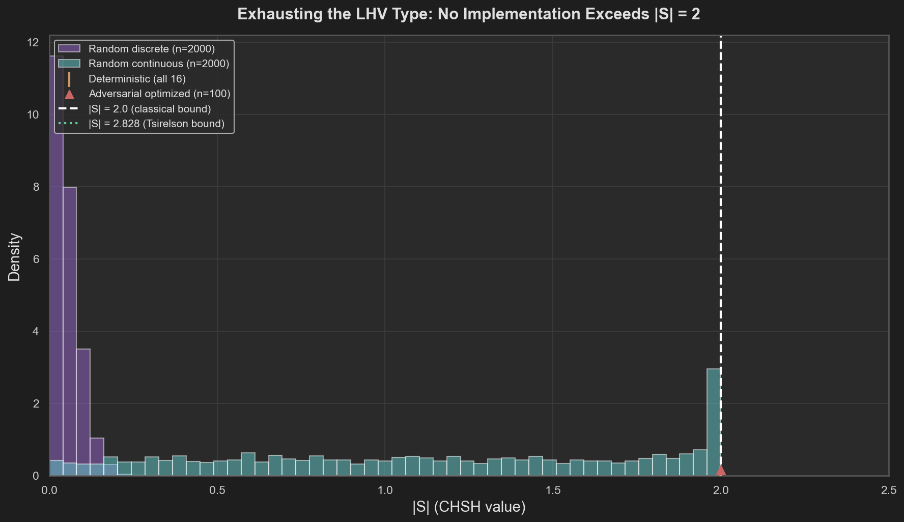
Figure 1. Distribution of |S| across thousands of LHV implementations. No strategy exceeds the classical bound |S| = 2, regardless of the structure of λ, the distribution, or the response functions. The adversarial optimizer hits the wall at exactly 2.
The factual picture is clear. Random strategies cluster well below the bound. Adversarial optimization reaches the bound but cannot exceed it. The deterministic strategies — the vertices of the convex set — all land at $|S| = 2$ exactly. The four categories searched different regions of the type’s inhabitant space: its vertices, its interior via random mixtures, its continuous extension, and its boundary via adversarial optimization. None escaped. The computational evidence is consistent with the theorem: $|S| \leq 2$ is not a tendency of typical implementations but an invariant of the type itself.
Beyond the Classical Bound
The proof established $|S| \leq 2$ as an invariant of the LHV type, and the computational search confirmed it across thousands of implementations. The bound is settled. Now let’s look at what nature actually produces.
The three-polarizer experiment
Before examining entangled pairs, consider a simpler experiment that reveals why the instruction-card model fails at a physical level. This involves single photons and polarizing filters — no entanglement. (You can try this yourself with three polarizing filters — cheap sunglasses or photography lenses work. The photon counts below correspond to the brightness of light you would see after each filter.)
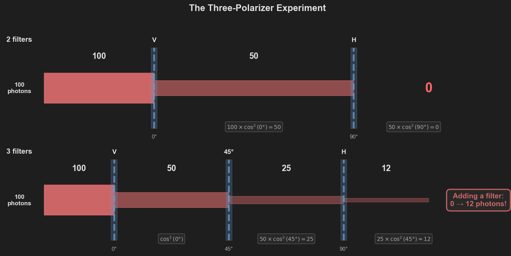
Two crossed polarizers block all light (top). Inserting a 45° filter between them lets ~12 photons through (bottom). Adding a filter increased throughput — something impossible if filters merely read pre-existing properties.
Two crossed polarizers. Send 100 unpolarized photons toward a vertical ($0°$) polarizer. On average, half pass through — the polarizer transmits the component of polarization aligned with its axis. That gives us 50 photons, now vertically polarized. Send those 50 into a horizontal ($90°$) polarizer. Malus’s law gives the transmission probability as $\cos^2(\Delta\theta)$, where $\Delta\theta$ is the angle between the photon’s polarization and the filter axis:
$$ 50 \times \cos^2(90°) = 50 \times 0 = 0 \text{ photons} $$Nothing gets through. Crossed polarizers block everything. So far, no surprises.
Now insert a 45° filter between them. Same 100 unpolarized photons hit the vertical polarizer — 50 pass, now vertically polarized. These 50 hit the new 45° filter:
$$ 50 \times \cos^2(45°) = 50 \times \tfrac{1}{2} = 25 \text{ photons} $$Those 25 are now polarized at 45° (the filter resets their polarization to its own axis). They hit the horizontal filter:
$$ 25 \times \cos^2(45°) = 25 \times \tfrac{1}{2} \approx 12 \text{ photons} $$We went from 0 to 12 by adding a filter. Think about what the instruction-card model predicts here. If each photon carried a card with predetermined pass/fail values at every angle, then each filter would simply read the card and either pass or block. Adding a third filter would mean one more gate to fail at. Throughput could only decrease or stay the same — never increase.
But the 45° filter does not read the photon’s polarization — it resets it. After passing the 45° filter, the photon is repolarized at 45°, regardless of what it was before. It now has a fresh $\cos^2(45°)$ probability of passing the horizontal filter. The filter did not check a pre-existing property; it prepared a new state.
This is the core distinction between the LHV type and quantum mechanics. In the LHV type, measurement reveals what $\lambda$ already determined — it is a lookup. In quantum mechanics, measurement projects the state onto a new basis — it is a transformation. The three-polarizer experiment makes this distinction visible with a beam of light and three pieces of plastic. And it is the same mechanism that makes Bell inequality violation possible: if measurement created new state rather than reading old state, the correlations between entangled pairs are not constrained by what any pre-existing card could have specified.
Entangled pairs violate the bound
The three-polarizer experiment involves single photons — no entanglement, no Bell inequality. But it exposes the physical mechanism. Now apply the same logic to entangled pairs, where the violation is quantitative.
For entangled photon pairs, quantum mechanics predicts that the probability Alice and Bob get different outcomes when their polarizers differ by angle $\Delta\theta$ is:
$$ P(\text{disagree}) = \sin^2(\Delta\theta) $$This is not a guess — it follows from the Born rule applied to the entangled state. Now plug these predictions into the Bell inequality we derived from the instruction cards:
$$ P(\text{disagree at } 0°,60°) \leq P(\text{disagree at } 0°,30°) + P(\text{disagree at } 30°,60°) $$Evaluate at our three angle separations:
- $P(\text{disagree at } 30° \text{ apart}) = \sin^2(30°) = \frac{1}{4}$
- $P(\text{disagree at } 60° \text{ apart}) = \sin^2(60°) = \frac{3}{4}$
The inequality requires:
$$ \frac{3}{4} \leq \frac{1}{4} + \frac{1}{4} = \frac{1}{2} $$But $\frac{3}{4} > \frac{1}{2}$. Violated by 25 percentage points.
In concrete counts. Out of 1,000 entangled pairs measured at $0°$ vs $60°$, quantum mechanics predicts 750 disagreements. Any instruction-card model can produce at most 500. The gap is 250 pairs — not a statistical fluctuation, but a structural impossibility.
Why the cards fail
The inequality is a theorem, not an approximation. No amount of cleverness in designing instruction cards can circumvent it, because it follows from the logical structure of pre-assigned values.
The deeper reason is geometric. The best any instruction-card model can do is a straight line: disagreement grows proportionally with angle, from 0 at $0°$ to 1 at $90°$. Quantum mechanics predicts disagreement rates that follow a $\sin^2(\Delta\theta)$ curve — which starts below the line at small angles (growing slowly), crosses it at $45°$, and then rises above it at large angles (steepening rapidly). The violation lives in that steepening: past $45°$, the quantum curve climbs faster than any classical mixture can follow.
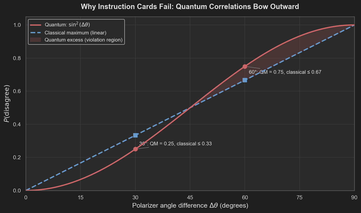
Disagreement probability vs polarizer angle difference. The quantum prediction (red, sin²Δθ) crosses above the classical maximum (blue dashed, linear) beyond 45°. At 30° the quantum disagreement (0.25) is below the classical bound (0.33) — the cards can accommodate it. At 60° the quantum disagreement (0.75) exceeds the classical bound (0.67) — no mixture of instruction cards can reproduce this. The shaded region is structurally inaccessible to any local hidden-variable model.
This is the same lesson as the three-polarizer experiment: measurement is not revealing a pre-existing property. If it were, the correlations would obey the instruction-card bound. They do not. The $\sin^2$ curve — which arises from quantum projection, the same mechanism that lets a 45° filter reset a photon’s polarization — steepens past $45°$ and rises above the classical envelope because it encodes correlations that no lookup table can produce.
The Quantum Type
Quantum mechanics assigns probabilities through a different mechanism.
In the classical model, probabilities compose directly:
$$ P(A, B \mid a, b) = \int P(A \mid a, \lambda) \, P(B \mid b, \lambda) \, d\mu(\lambda) $$In quantum mechanics, the fundamental objects are amplitudes, not probabilities. For a quantum state $|\psi\rangle$, the probability of an outcome is obtained via the Born rule:
$$ P(\text{outcome}) = |\langle \text{outcome} | \psi \rangle|^2 $$The squaring — the passage from amplitude to probability — is a nonlinear operation. Amplitudes can interfere (add constructively or destructively) before the probability is extracted. This interference occurs before probabilities are computed, which changes the set of achievable correlations. Classical models combine probabilities over hidden states. Quantum models combine amplitudes and only then derive probabilities. These operations produce different correlation structures. This means the joint distribution $P(A, B \mid a, b)$ for an entangled state does not factorize through any shared classical variable.
For the singlet state $|\psi^-\rangle = \frac{1}{\sqrt{2}}(|01\rangle - |10\rangle)$, the correlation between spin measurements at angles $\theta_a$ and $\theta_b$ is:
$$ E(\theta_a, \theta_b) = -\cos(\theta_a - \theta_b) $$This follows directly from the Born rule applied to projective measurements on the entangled state. The key mechanism is that the singlet state encodes correlations in amplitude space, and these correlations survive the Born rule in a form that no classical factorization can reproduce.
The contrast is visible in code. A classical LHV model computes correlations by averaging over shared lookup tables. The quantum singlet state computes them through the Born rule — amplitudes interfere before probabilities are extracted:
# Classical: correlations from shared instruction cards
def classical_correlation(a, b, cards, weights):
    return sum(w * card[a] * card[b] for card, w in zip(cards, weights))
    # Each term is ±1. The average is bounded by the extremes: |E| ≤ 1.
    # Combined into CHSH: |S| ≤ 2.

# Quantum: correlations from amplitude interference (Born rule)
def singlet_correlation(theta_a, theta_b):
    return -np.cos(theta_a - theta_b)
    # Not a lookup or an average over hidden data —
    # a direct consequence of projecting the entangled state.

def singlet_joint_probabilities(theta_a, theta_b):
    delta = theta_a - theta_b
    return {
        (+1, +1): np.sin(delta/2)**2 / 2,  # both same
        (+1, -1): np.cos(delta/2)**2 / 2,  # opposite
        (-1, +1): np.cos(delta/2)**2 / 2,  # opposite
        (-1, -1): np.sin(delta/2)**2 / 2,  # both same
    }
Specifically, for the singlet state there is no decomposition:
$$ P(A, B \mid a, b) \neq \int P(A \mid a, \lambda) \, P(B \mid b, \lambda) \, d\mu(\lambda) $$for any hidden variable $\lambda$ and any local response functions. This is Bell’s theorem: the factorization demanded by the LHV type signature is incompatible with the observed correlations.
Quantum violation: $|S| = 2\sqrt{2}$
At the optimal CHSH angles — $a_1 = 0°$, $a_2 = 90°$, $b_1 = 45°$, $b_2 = 135°$ — the singlet state produces:
$$ |S| = 2\sqrt{2} \approx 2.828 $$This is the Tsirelson bound [4]: the maximum CHSH violation achievable by any quantum state. It exceeds the classical bound of 2 by a factor of $\sqrt{2}$.
We verify this by simulating projective measurements on the singlet state using the Born rule. For each of the four setting pairs, we sample 100,000 measurement outcomes from the joint distribution and estimate $E(a, b) = \langle A \cdot B \rangle$.
The computation uses the same CHSH formula — the only difference is the correlation source:
a1, a2 = 0, np.pi/2          # Alice: 0° and 90°
b1, b2 = np.pi/4, 3*np.pi/4  # Bob:  45° and 135°

S = (singlet_correlation(a1, b1) - singlet_correlation(a1, b2)
   + singlet_correlation(a2, b1) + singlet_correlation(a2, b2))
# S = -2√2 ≈ -2.828
# |S| = 2.828 > 2 — the classical bound is violated.
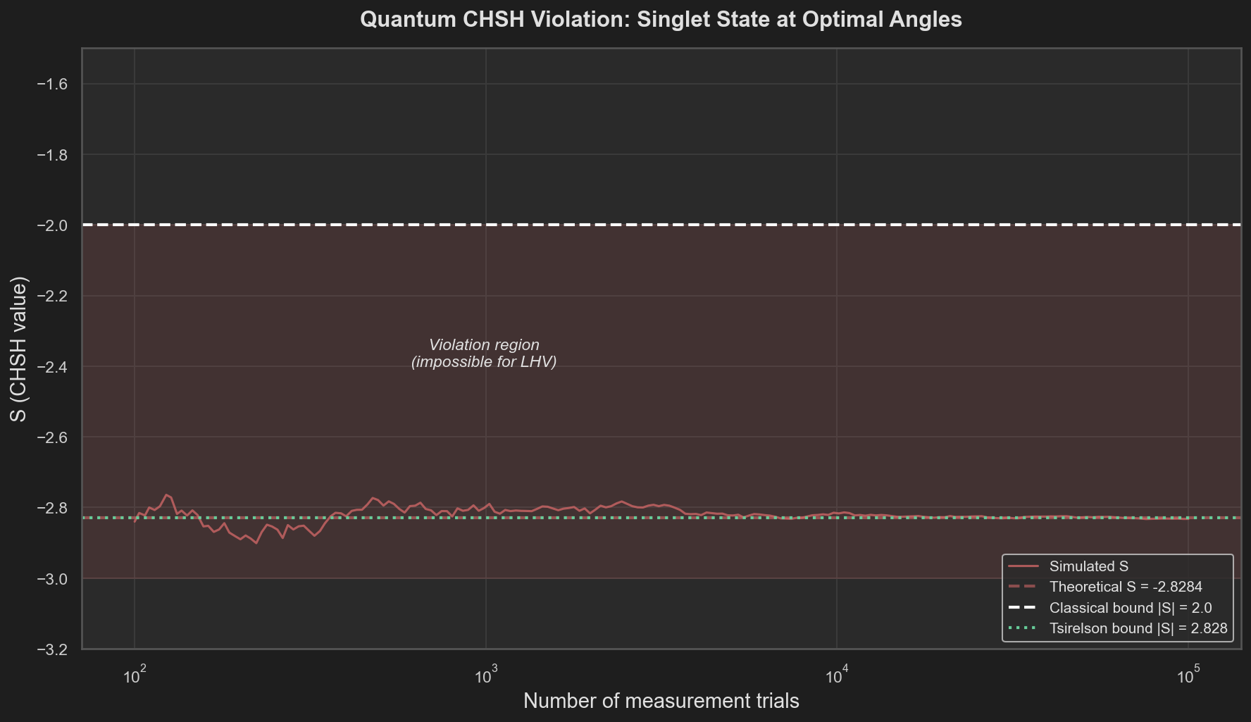
Figure 2. Convergence of simulated S toward the theoretical value S = −2√2 as the number of measurement trials increases. The estimate enters the violation region (|S| > 2) within a few hundred trials and stabilizes near the Tsirelson bound.
The simulation converges to the theoretical value. The violation is not marginal — the quantum $|S|$ exceeds the classical bound by over 40%. With sufficient measurement statistics, the violation is unambiguous.
Interactive: CHSH Angle Sweep
The magnitude of the CHSH violation depends on all four measurement angles. The interactive visualization below lets you vary the angles and watch $|S|$ update in real time.
The main curve sweeps Bob’s angle $b_1$ from $0°$ to $360°$ while holding the other three angles fixed (adjustable via sliders). The classical bound $|S| = 2$ and the Tsirelson bound $|S| = 2\sqrt{2}$ are marked for reference.
At the default settings ($a_1 = 0°$, $a_2 = 90°$, $b_1 = 45°$, $b_2 = 135°$), the quantum $|S|$ sits at $2\sqrt{2}$. As you move the sliders, observe that:
- The violation region is not a single point but a continuous range of angle configurations
- The maximum violation occurs when the four angles are evenly spaced at $45°$ intervals
- No angle configuration produces $|S| > 2\sqrt{2}$ — the Tsirelson bound is a quantum-level type constraint, just as $|S| \leq 2$ is a classical one
Non-Embeddability
We can now state the conclusion precisely.
The LHV type defines a class of programs:
$$ \text{LHV} = \left\{ (A, B, \mu) \;\middle|\; A : \text{Setting} \times \Lambda \to \{+1,-1\}, \; B : \text{Setting} \times \Lambda \to \{+1,-1\}, \; A \perp\!\!\!\perp b, \; B \perp\!\!\!\perp a \right\} $$The CHSH inequality $|S| \leq 2$ is an invariant of this type. Any program in LHV satisfies it. This was established by proof and verified computationally across thousands of implementations.
Quantum mechanics produces correlations with $|S| = 2\sqrt{2}$. These correlations are observable, reproducible, and experimentally confirmed [5].
The implication is a non-embeddability result: the quantum correlations cannot be realized by any program of the LHV type. This result does not depend on the choice of hidden variable. It is a proof that no hidden variable with the LHV dependency structure can reproduce the data.
The failure is in the factorization constraint. It is not that $\lambda$ is the wrong variable, or that the distribution is wrong, or that the response functions are not clever enough. The entire type is wrong. No extension of $\lambda$ within this factorization constraint can close the gap. The space of programs defined by local hidden variables and classical probability composition does not contain any program that produces the observed correlations.
This is the same pattern we encountered in The Models We Choose Define the Worlds We Can See: representational constraints determine what dynamics can be expressed. An ODE cannot express network-dependent contagion. An LHV model cannot express quantum correlations. In both cases, the limitation is not in the parameter values — it is in the model’s type signature.
Closing
Bell’s theorem is a constraint derivable from a dependency pattern. If your model is local and classical, it satisfies $|S| \leq 2$. If the world produces $|S| > 2$, your model does not describe the world. Not because it needs better parameters, but because it inhabits the wrong type.
Quantum mechanics works because it computes in amplitude space. Amplitudes interfere before probabilities are extracted. This interference produces correlations that no classical factorization can replicate. The Born rule’s nonlinearity — the squaring that converts amplitudes to probabilities — creates a gap between what classical programs can produce and what quantum systems actually produce.
Bell’s theorem identifies a mismatch between the structure of classical probabilistic models and observed correlations. Quantum mechanics resolves this by operating in a different representational space.
Experiments
The computational experiments supporting this essay are available in the project repository:
- Experiment 1 – Exhausting the Type: LHV Ensemble – Thousands of local hidden-variable implementations, all bounded by |S| = 2.
- Experiment 2 – Quantum Violation: Singlet State Simulation – Born rule measurements on the singlet state produce |S| = 2√2.
- Experiment 3 – Interactive Sweep: CHSH Angle Explorer – Interactive Plotly visualization of CHSH value vs measurement angles.
Full source code
The complete implementation – including LHV models, quantum simulation, adversarial optimization, and all plotting – is available in the experiments/bells_inequality/ directory. Run it with:
python run_experiment.py --experiment all
References
Clauser, J. F., Horne, M. A., Shimony, A., & Holt, R. A. (1969). “Proposed experiment to test local hidden-variable theories.” Physical Review Letters, 23(15), 880-884.
Bell, J. S. (1964). “On the Einstein Podolsky Rosen paradox.” Physics Physique Fizika, 1(3), 195-200.
Wadler, P. (1989). “Theorems for free!” Proceedings of the Fourth International Conference on Functional Programming Languages and Computer Architecture, 347-359.
Tsirelson, B. S. (1980). “Quantum generalizations of Bell’s inequality.” Letters in Mathematical Physics, 4(2), 93-100.
Aspect, A., Dalibard, J., & Roger, G. (1982). “Experimental test of Bell’s inequalities using time-varying analyzers.” Physical Review Letters, 49(25), 1804-1807.
Einstein, A., Podolsky, B., & Rosen, N. (1935). “Can quantum-mechanical description of physical reality be considered complete?” Physical Review, 47(10), 777-780.
This essay is part of the SHARC Theory research project.